Format Locked or Unlocked Cells

This post explores options for formatting cells that are locked, or unlocked, in an Excel worksheet.

Scenario

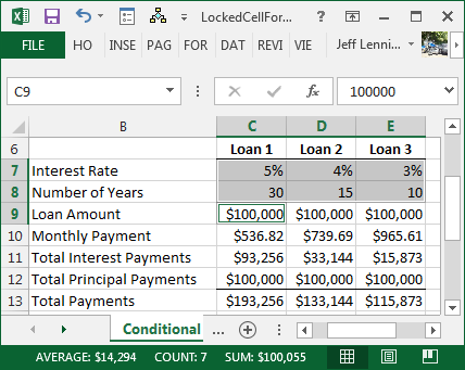
Let’s pretend we have a worksheet that helps a user compare three different loans. The user is required to enter information, such as interest rate and number of years, into designated input cells, but shouldn’t be allowed to type into the formula cells, such as the monthly payment cell. Thus, we have two objectives (1) identify the input cells for the user and (2) lock the non-input cells.

Locking the non-input cells is relatively easy since they are already locked. Wait, what? Yep…all cells, in all worksheets, in all workbooks, by default are locked. Wait, what? Yes, all cells are locked by default…however…the locked attribute isn’t enforced until we activate worksheet protection. So, a more precise way to describe our task is to say that we need to unlock the input cells. To do so, we start by selecting them, as shown in the screenshot below:

With the input cells selected, we unlock them by unchecking the Locked checkbox on the Protection tab of the Format Cells dialog or clicking the following Ribbon command:

• Home > Format > Lock Cell

The Lock Cell button is a toggle button, so, selecting it repeatedly switches between locking and unlocking the selected cells.

Once the input cells are unlocked, we activate worksheet protection by selecting the following Ribbon icon:

• Home > Format > Protect Sheet

At this point, the user can enter values into the unlocked input cells, however, Excel will prevent the user from typing into the locked cells. In order to update the worksheet for the changes below, we’ll turn off worksheet protection for now by selecting the following Ribbon icon:

• Home > Format > Unprotect Sheet

In order to help the user identify the input cells, we’ll highlight them. As with just about anything in Excel, there are several ways to accomplish this task. The two we’ll cover are conditional formatting and cell styles.

Option 1: Conditional Formatting

The first idea is to use the conditional formatting feature to format the unlocked cells. In order to accomplish this task, we’ll use a formula to format the cells. If you are unfamiliar with this technique, please refer to the Conditional Formatting Based on Another Cell post.

The formula we’ll need to write should return TRUE when a cell is unlocked. This can be accomplished with the CELL function. The CELL function syntax follows:

=CELL(info_type, [reference])

Where:

• info_type is the type of cell information you’d like, such as the color, format, or protection status. See Excel’s help system for options.
• [reference] is the cell you’d like information about.

We’ll use the CELL function to determine if the cell is locked or unlocked. If it is locked, the function returns 1 (TRUE) and if unlocked the function returns 0 (FALSE). For example, if we wanted to find out if cell A1 is locked, we would use the following formula:

=CELL("protect",A1)

If the formula returns 1, we know it is locked. If it returns 0, it is unlocked.

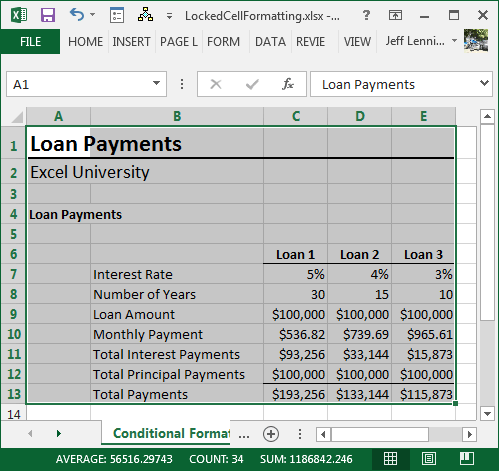
To apply the conditional formatting rule, we begin by selecting the range of cells we want Excel to conditionally format, as illustrated in the screenshot below:

Using the active cell (A1) in the conditional formatting formula, we could use the following formula to highlight locked cells:

=CELL("protect",A1)

If locked, it would return 1 (TRUE). If unlocked, it would return 0 (FALSE). However, since our goal is to format the unlocked cells, rather than the locked ones, we need to write a formula that returns TRUE when unlocked. We can do this with a simple comparison formula as follows:

=CELL("protect",A1)=0

We create a new conditional formatting rule that uses a formula to determine which cells to format. We enter the formula and define the desired formatting, as shown below:

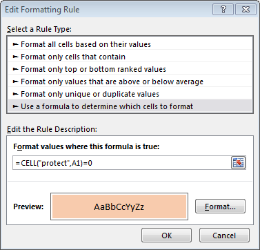
Now, the unlocked input cells are highlighted, as shown below:

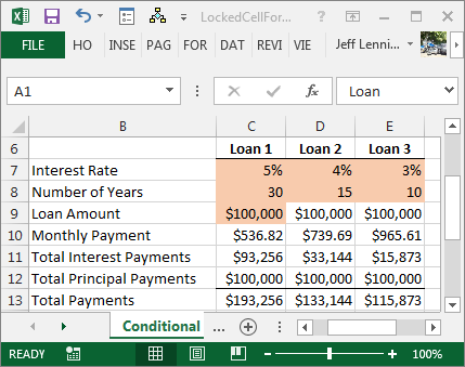
At this point, locking or unlocking a cell within the conditionally formatted range will cause Excel to apply the desired format.

This approach is essentially a two-step process whereby we manually unlock a cell and then Excel applies the proper format. Alternatively, we could manually format the input cell and unlock it in a single step using cell styles. This is the approach I prefer and use in practice. Let’s check it out.

Option 2: Cell Styles

A style is a set of formatting instructions. Rather than manually format each element of a cell, we can apply a style to the cell. If we change the style definition, all cells with that style are updated accordingly.

Microsoft has designed a style specifically for input cells called Input. We can easily apply the Input cell style to cells by using the following Ribbon icon:

• Home > Styles > Input

The Input cell style includes information about the fill and font color, but not the protection status. However, we can easily update the style to include information about the protection status. Right-click the Input cell style Ribbon icon and select Modify to open the Style dialog. Check the Protection checkbox as shown below:

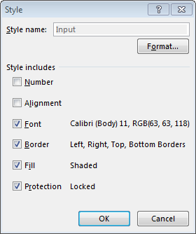
After checking the Protection checkbox, click the Format button to open the Format Cells dialog. Uncheck the Locked checkbox on the Protection tab as shown below:

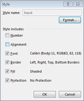
The Style dialog will update to indicate No Protection, as shown below:

Now, whenever you apply the Input cell style to a cell, it is both formatted and unlocked at the same time.

To enforce this setting, turn on worksheet protection as follows:

• Home > Format > Protect Sheet

Now, the user can change values in the input cells, but, when they try to change a formula cell they are greeted with an error alert, as shown below:

If you have an additional approach, please post a comment below, I’d love to hear more about it!

Additional Resources

• Download sample file: LockedCellFormatting
• PMT function post: Calculate the Payment of a Loan with PMT
• Detailed steps for cell style protection: Cell Styles and Worksheet Protection