Excel Calendar Table
When you need to summarize values by date groups, a calendar table can be helpful. While Power Pivot has a button that will automatically create a new date table (shown in this post), Excel doesn’t have a similar command. So, in a recent Q&A session, Michael asked how to get that Power Pivot calendar table into Excel. While we could copy/paste the static values or display it with a PivotTable, we can create an Excel calendar table with just a few functions. Thanks for your question!
Objective
Before we get to the mechanics, let’s take a look at a calendar table created automatically in Power Pivot by clicking the Design > Date Table > New command:

As you can see, it contains a Date column, and then a series of calculated columns that display various values we can use in our reporting such as Year, Month number, Month name, Day, and so on.
So, our objective is to create something similar in Excel.
Walkthrough
We’ll create our calendar table using these steps:
- Create the date column
- Create standard calendar columns
- Create custom calendar columns
Let’s get to it.
Create the date column
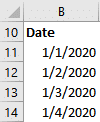
The first step is to create the Date column. It is essentially a list of all dates that spans our data range. It needs to contain one row per date and it needs to include all dates. Basically, a list like this:
As this is Excel, there are many ways to create this column. One way is to enter the start date into a cell and then drag the fill handle (tiny square in lower right corner of cell) down the desired number of rows.
You could also select the starting date cell and a bunch of cells below it, and use the Home > Fill > Series command.
Another way is to type the starting date into a cell, and then use a formula to add 1 to it. Something like =B1+1 or similar. You can then fill that formula down.
If your version of Excel includes the SEQUENCE function, you could enter the start date and then reference it inside the SEQUENCE function.
And there are no doubt many other ways to create such a column.
Regardless of how you create the date column, when you are done you should have a column of dates that covers the date range of your data. It should include one and only one row for every date and should not skip any dates. You’ll probably want it to start on the first day of the first month of your year and end on the last day of the last month of your year in case you need any calculations based on number of days.
This set up will help ensure that your lookups will work on all transaction dates. Plus, it provides the flexibility to accommodate subsequent formulas you may need down the road.
With the Date column complete, we can then add the standard calendar columns.
Create standard calendar columns
Excel provides a wide variety of date related functions that can help here. If we wanted to create the standard calendar columns that Power Pivot creates, we’ll need to compute these columns:
- Year
- Month number
- Month name
- MMM-YYYY
- Day of week number
- Day of week name
Let’s just walk through them one at a time.
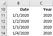
Year
To create the year column as numbers, we can use the YEAR function like this:
=YEAR(B11)
When we fill the formula down:
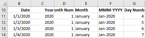
Month number
For month number, we can use:
=MONTH(B11)
Fill it down and:

Month name
For month name, we can use the TEXT function. If you’ve not explored it before, it enables you to format a value based on the format code. The codes for dates are:
- m – month number without leading zero (1)
- mm – month number with leading zero as needed (01)
- mmm – three letter month abbreviation (Jan)
- mmmm – full month name (January)
- d – day number without leading zero (1)
- dd – day number with leading zero as needed (01)
- ddd – three letter day abbreviation (Mon)
- dddd – day name spelled out (Monday)
- yy – two digit year
- yyyy – four digit year
So, we can create a column with the full month name like this:
=TEXT(B11, "mmmm")
Fill it down and:

MMM-YYYY
We can once again use the TEXT function for this column:
=TEXT(B11, "mmm-yyyy")
Fill it down and:

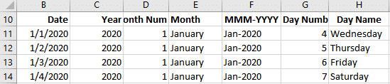
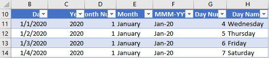
Day of week number
We can use the WEEKDAY function like this:
=WEEKDAY(B11)
Fill it down and:
Day of week name
Day of week name can be created with the TEXT function like this:
=TEXT(B11, "dddd")
Fill it down and:
We could optionally convert the ordinary range into a Table by using the Insert > Table command. This will make it easier to reference via the Table’s name (like Table1) and the formulas will fill down automatically.
With our calendar table (Table1) in place, we can then use a lookup function such as VLOOKUP to retrieve values from it as needed.
For example, if we had some transactions like this:

We could use a lookup function such as VLOOKUP to retrieve the day name from our calendar table. In cell F7 we could use:
=VLOOKUP(C7, Table1, 7, 0)
Fill it down and bam:

Depending on what we are working on, we could then use this Day Name helper column in our reports.
But, depending on our reports and what we are working on, we may need additional columns beyond the standard “calendar year” periods. Next, let’s explore custom calendar columns in case we need to reflect something like a fiscal quarter.
Create custom calendar columns
Let’s say we have a company with a fiscal year end date of June 30. We would like to create a Fiscal Quarter column, where months of Jul-Sep are Q1, Oct-Dec are Q2, Jan-Mar are Q3, and Apr-Jun are Q4. There are many formula options that we could use to create such a column.
One way is to simply create a lookup table based on month, like this (Table2):
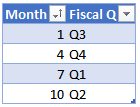
Note: must be sorted in ascending order by the Month column
We can then create a Fiscal Q column in our calendar table with a lookup function such as VLOOKUP like this:
=VLOOKUP([@[Month Num]],Table2,2,TRUE)
Bam:

Conclusion
This type of calendar provides an easy way to retrieve various date attributes in other areas of your workbook. Let me know what you think and if you have any other approaches or tips, please share by posting a comment below … thanks!
Sample File
Excel is not what it used to be.
You need the Excel Proficiency Roadmap now. Includes 6 steps for a successful journey, 3 things to avoid, and weekly Excel tips.
Want to learn Excel?
Our training programs start at $29 and will help you learn Excel quickly.
Outstanding reference Jeff, thank you… Very much appreciated…!!!
This is very helpful. You’ve just saved me a ton of time! Thank you!
Nice reminder of that fourth argument in VLOOKUP, thanks!