Dependent Drop Downs with FILTER
This post shows how to create multiple dependent drop downs using the FILTER function. These are also known as cascading or conditional drop downs, where the choices in a drop down depend on the selection made in a previous drop down. The technique presented enables you to create as many drop downs as you need, and there is no VBA coding needed.
Note: depending on your version of Excel, you may not have access to the FILTER, UNIQUE, or SORT functions. If not, check out this post which uses legacy functions or this post which uses slicers.
Objective
Before we get into the mechanics, let’s clarify our goal. We would like to create a series of dependent drop downs, where the choices available in a drop down depend on the selection made in a previous drop down.
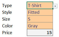
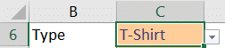
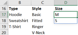
For example, we would like the user to pick a Type of shirt. Depending on the Type of shirt selected, the user will see various Style options. Depending on the selected Style option, the corresponding Size options are displayed, and so on. Perhaps something like this:
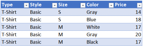
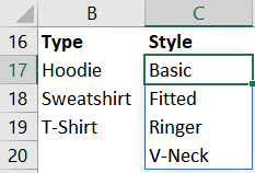
These configuration options all come from a single table, which stores all valid combinations. Perhaps something like this (Table1):
To create this, we’ll use a few functions (SORT, UNIQUE, FILTER) along with data validation.
Video
Narrative
We’ll build this using these steps:
- Create a drop down list
- Repeat for each drop down
- Retrieve related info
Let’s get to it.
Create a drop down list
We’ll perform three steps for each drop down:
- Create the list of choices
- Create the in-cell drop down
- Make a selection
We’ll ultimately repeat these steps for each subsequent drop down.
Create the list of choices
To create the list of choices, we’ll write a formula in an unused area of the worksheet.
Let’s start with the first drop down, which in our case is Type.
The first drop down has no dependencies, and thus will include the same list of choices all the time. Since the products table is named Table1, and the first drop down needs to provide a unique list of all items found in the Type column, we’ll use the following formula:
=UNIQUE(Table1[Type])
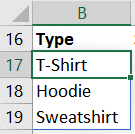
We write the formula into cell B17 and hit Enter. We see that the formula returns multiple results:
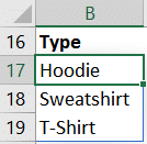
If we’d like the list to be sorted, we can include the SORT function in our formula like this:
=SORT(UNIQUE(Table1[Type]))
Now our list of choices is sorted, like this:
With our list of choices ready, we just need to get them into an in-cell drop down. For this, we’ll use Data Validation.
Create the in-cell drop down
We select the input cell, and use Data > Data Validation. We allow a list, and set the source to =$B$17# like this:
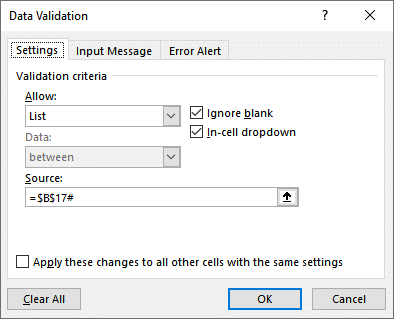
Note: the # tells Excel to include all results returned by the formula.
The input cell now contains a drop down with the list of choices.
Make a selection
Although we technically do not need to make a selection from the drop down right now, it will make the next step easier if we do. So, we select the input cell and pick any choice so that the cell is not empty, like this:
Note: the reason we make a selection is to avoid formula errors that could lead us to believe our formula is wrong.
Repeat for each drop down
Then, we perform these steps again for each subsequent drop down. We need to write a formula to create the list of choices, use data validation to create the drop down, and then make a selection so the cell is not empty.
But, there is a catch. Each subsequent list of choices depends on the choice made in the previous input cell. To accommodate this dependency, we’ll use the FILTER function.
Style Drop Down
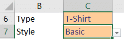
The next choice list is for Style. The choices for Style depend on the selection in the Type input cell. So, to create our list of Style choices, we use this formula:
=SORT(UNIQUE(FILTER(Table1[Style],Table1[Type]=C6)))
This basically tells Excel to return a sorted list of unique Style values where the Type column is equal to the selected Type in C6. We write the formula in C17 and hit Enter:
To get that list of choices into the Style input cell, we once again use Data Validation. This time, the source is =$C$17#. We expand the resulting Style drop down and make a selection so the cell is not blank:
The next input cell is for Size.
Size Drop Down
For Size, our list of choices depends on the values selected for Type and Style.
So, our FILTER function will show the list of Sizes where Type and Style values match. To use AND logic when we have multiple conditions, we use a multiplication operator * like this:
=SORT(UNIQUE(
  FILTER(Table1[Size],(Table1[Style]=C7)*(Table1[Type]=C6))
))
Note: to use OR logic instead of AND logic, we would use the addition operator + instead of the multiplication operator.
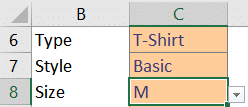
We write the formula into cell D17 and hit Enter:
To create the drop down, we use Data Validation and set the source =$D$17#. We expand the resulting drop down and make a selection, like this:
So far so good … we just have one final drop down.
Color Drop Down
The final drop down for this illustration is color, but you can continue using this same technique for as many drop downs as needed.
Our formula to create the choices includes conditions for Type, Style and Size:
=SORT(UNIQUE(
  FILTER(Table1[Color],
    (Table1[Size]=C8)*(Table1[Style]=C7)*(Table1[Type]=C6)
    )
))
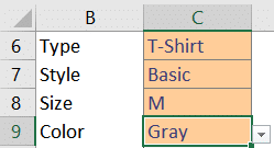
We write the formula into E17 and hit Enter:

We use Data Validation to create the drop down, and set the source =$E$17#. We make a selection:
Now that we have created the dependent drop downs, we can optionally return related values.
Retrieve related info
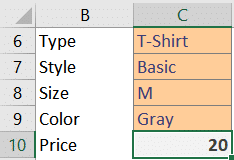
In our case, once the user has selected the Type, Style, Size, and Color, we’d like Excel to return the related Price.
Once again, we’ll turn to the FILTER function. We write the following formula into C10:
=FILTER(Table1[Price],
  (Table1[Color]=C9)*(Table1[Size]=C8)*(Table1[Style]=C7)*(Table1[Type]=C6)
)
We hit Enter, and bam:
Note: if the products table contained multiple matching rows, we can aggregate the results with a helper function such as SUM, MIN, MAX, TEXTJOIN, AVERAGE, COUNT, and so on.
If you see any #CALC! errors, it probably means that the dependent input cells are blank, or that the options selected don’t have related values. This could happen if you change the selection in the first input cell and don’t pick valid options from the updated drop downs for the subsequent cells.
Conclusion
I think we accomplished our goal. We created a series of dependent drop downs. We used a few functions (FILTER, UNIQUE, SORT) and data validation. Let me know what you think by posting a comment below … thanks!
Sample file
Excel is not what it used to be.
You need the Excel Proficiency Roadmap now. Includes 6 steps for a successful journey, 3 things to avoid, and weekly Excel tips.
Want to learn Excel?
Our training programs start at $29 and will help you learn Excel quickly.
Brilliant, as always you make the solution to a complex problem look so easy.
Thanks 🙂
Very informative, nice job.
This is most Excel lent! Clear and concise 🙂 Is there a way to make the sort/unique/filter work as a data validation rule?
George,
Sorry this is from so long ago…. You had asked ‘Is ther a way to make sort/filter work as a data validation rule?” I had the same question. Did you find an answer?
Wonderful!
Apparently, creating creating dependent drop downs with FILTER is much easier and compact than other options (especially those where data are stored in one table and we had to create multiple dynamic named ranges for 1st row, last row, etc. – that exercise from graduate course was brutal).
I need help. This was very informative! But it still gave me problems. I have 3 manufacturing lines, producing multiple part numbers on each. Some of the part numbers are run on both lines 1 and 3 but not on line 2, some on lines 2 and 3, but not on line 1. I’m trying to find a way to get the part numbers to be listed in a drop-down list depending on which line number is selected from the first drop-down list. Can you help me with that? I would be most appreciative! Thank you so much!
Jeff, you saved me with this today. I had taken your Excel University CPE classes before and thought you may have a resource on your blog that would help solve my problem. As luck would have it, this expansion on data validation perfected the time-saving project I was working on for my boss. We’re all going to be so much more efficient thanks to your instructions! This made my whole week.
Yay … glad I could help 🙂
Impressive clarity and structure of your solution! Thanks!
Hi
I am working with a table where I would like to implement this useful function but my table works horizontally rather than vertically. Is it possible to do this with rows rather than the table headings? For example Table1[syte} would be Table1[row8]?
Thanks in advance.
I wish I would have come here first! Spent so many hours trying to figure out this issue and countless sites/blogs. You made it so easy and it works to perfection! Thanks for posting!
Thanks for your kind note and I’m glad it helped!
How would I remove the #CALC error if let’s just say I only wanted to order 1 clothing item, but I could choose up to ten? The other 9 spots give me a #CALC! error, becuase nothing is chosen. It is also ruining my total sum formula. How do I sum if with a #CALC! ERROR?
Please disregard the above question. I was able to figure it out. However, can I make this dynamic? Looking to make dynamic for 9 9other spots/ choices/
Hi Jeff!
Thanks for work and it is very helpful kudos for your time and effort!
In this context, I have used this sheet Microsoft 365 and its working fine. However, the same is not working in excel 2019 has there are no functions such as SORT or Filter in ec; 2019 . Kindly request how to execute the same in 2019 or below.
Thanks much in advance
Reg , Sri
Excellent! Thanks for your post!
Brilliant!
Thank you.
Hi,
I came up with a similar solution which you have helped me to complete. My challenge now is to incorporate this logic into a dynamic form. So, instead of having the filter functions reference a fixed cell I want them to reference the cell next to them, so that each time I select a cell in, say, column B, the validation options next to it in column C will vary dynamically.
There are examples on the web with named lists, but they mostly use named ranges. I don’t want to have to add new named ranges every time my source table varies – and there would be too many anyway.
I think I am close, but Excel doesn’t seem to like filter functions in its source range. I will keep trying, but if you have any ideas I would be very appreciative.
This is exactly what I’m looking for – have you figured this out?
Jeff,
I had the same question that George had….
Is there a way to make the sort/unique/filter work as a data validation rule?
I replied, but since it’s so long ago, I’m not sure George will be reached. Do you have an answer to George’s question?
A data validation drop down list is tied to a range of cells, meaning, you point the data validation list to the results of the formula. To my knowledge, at this time, Excel doesn’t support embedding the formula into the data validation formula in order to avoid referring to a cell range.
If I misunderstood your question, just reply … thanks!
Hi and thanks to all specially to the author. Although I have a question/doubt: I have it all working as it should with the exception that the “old” value persists on the cell and only after changing the initial filters, it then, upon open the dopdown, show the available values
Jeff,
Thanks for posting your example, I agree with many that posted – your example is much clearer yet more concise than many of the other experts. As I studied your example, I initially thought you had the solution I needed, but I haven’t been able to expand on it.
My scenario is I have an input sheet where designers identify the parts needed for a given design. On that sheet each row is a part to be ordered, and each column contains part attributes (like your example). Sometimes the designs will have 10 parts and sometimes hundreds. I have separate tab with all my valid parts and their attributes. I also created ranges for the table and key columns.
Where I run into an issue with you example is with the Drop-Down Prep section. Your example seems to only support 1 series of drop downs (i.e., 1 part or product).
In our scenario the designer begins be selecting a Manufacturer in Column A. The Data Validation – Drop-Down for that Column works properly. The designer then selects the Part Number which has a list that is dependent on the manufacture selected. Very similar to your example.
This is how I was originally started off doing my Data Validation:
=OFFSET(All_Parts,MATCH(A5,All_Parts_Manufact,0),3,COUNTIF(All_Parts_Manufact,A5),1)
The issue I have with this approach is it only works if the data in the source parts table is already sorted. In our scenario, the parts list may not always remain sorted.
Is there a way to combine our two approaches into a simpler, concise one which also support multiple rows being added to the input sheet and support additions/subtractions to the Parts List?
Thanks
I think I know what you are trying to do. May I suggest that you have a separate list of the data types via a formula such as this =SORT(UNIQUE(FILTER(SourceDataTableColumn,SourceDataTableColumn””)))
Then when people enter the data into the source data table, it will automatically sort and list those in that separate list (which cannot be a table – but you can name that column and use the column name All_Parts_Manufact as the data validation. In the SourceDataTableColumn you can set the data validation to the list and can allow for people to enter new parts (or not) depending on how you want to do that. Just a thought.