Custom Conditional Formatting Rules

Today, we will look at using conditional formatting with formulas, data validation, and comparison formulas.  Think you are up for it?  Let’s do this thing.

Let’s say we have a worksheet that computes the payment of a loan.  We can use the PMT function to easily accomplish this task.  The PMT function requires three arguments to compute the payment amount.  The function requires the loan amount, the interest rate, and the term.  The thing about the payment function is that the unit of time must be consistent.  That is, if you want to compute the monthly payment, then the interest rate must be expressed as a monthly interest rate, and the term must be expressed as the number of months.  If you  want the annual payment amount, then you need to express the interest rate as an annual rate and the term as the number of years.

If we want to make the worksheet easy for our user, then we would want to allow the user to pick between months and years.  We set up a Payment Period input cell, and provide the user with an in-cell dropdown to pick Monthly or Annual.  (An in-cell dropdown is easily created with the Data Validation feature; Data > Data Validation.)

Typically, interest rates are expressed as annual rates, so we’ll ask the user to enter the annual interest rate and then convert it to a monthly rate if needed.  As far as the term goes, we could set up one input cell to allow the user to enter the term, and that would be just fine.  However, we prefer to set up two input cells so that if the user wants to do a monthly payment, the user can enter the number of months into the Term (months) input cell.  If the user wants to do an annual payment, the user can enter the number of years into the Term (years) input box.  This idea is illustrated in the screenshot below.

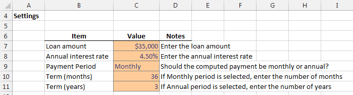
The thing about our settings area is that it may be confusing for the user since the user may not be sure if an entry is required in both Term input cells.

The formula that computes the payment amount uses the Term (months) value if the user picks Monthly, and uses the Term (years) value if the user picks Annual.  We should make it clear to the user which input cells are currently being used by the formula. The payment formula uses an IF function to perform different math based on the selected payment period.  If the user selects a Monthly Payment Period, then the formula uses the value in the Term (months) input cell C10.  If the user selects an Annual Payment Period, then the formula uses the value in the Term (years) input cell C11.

The payment formula is below:

=-IF(C9=”Annual”,PMT(C8,C11,C7),PMT(C8/12,C10,C7))

If the Payment Period is “Annual”, then a PMT function that uses the C11 term input cell is used, otherwise, a PMT function that uses the C10 term input cell is used.

This leads us to the reason why we are here.  We can use a simple conditional formatting rule that makes is clear for the user which term input cell to enter a value into, and, which input cells are being evaluated by the formula.

Basically, if the user picks an Annual Payment Period, then we want the user to enter a value into the Term (years) input cell.  So, we will make the Term (months) input cell dimmed out with gray formatting.  Likewise, if the user picks a Monthly Payment Period, then we want the user to enter a value into the Term (months) input cell.  So, we will make the Term (years) input cell dimmed out with gray formatting.

On the Term (months) input cell, we want to set the formatting to gray if the Payment Period is equal to Annual. So, we select the Term (months) input cell, and apply the following conditional formatting rule by heading to the Conditional Formatting > New Rule ribbon command:

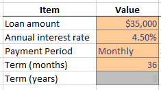
First, notice that we selected “Use a formula to determine which cells to format.”  This setting allows us to enter any formula or function that returns a TRUE or FALSE value.  If it returns TRUE, then the formatting is applied.  In our case, we just use a simple comparison formula.  =$C$9=”Annual” which returns TRUE if the value in C9 is equal to “Annual.”  If the user selects an Annual Payment Period, then the Term (months) input cell is dimmed gray.  You could pick any formatting you like by clicking the Format button.  I picked a gray font with a light gray cell fill.

The results are shown below.

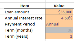
We apply a similar conditional formatting rule to the Term (years) input box, shown below:

And, the results are shown below:

This simple idea of using conditional formatting to make it clear for the user which input cells are active and not active can be used in a wide variety of situations.

If you’d like to download the working file, use the link below.

Formatting