Conditional Formatting With Data Validation

In today’s Excel University blog post, we’re going to explore the incredible combination of the Conditional Formatting and Data Validation features in Excel. I was recently asked the following question: How do I highlight matching customers on one worksheet based on the customer selected in a data validation drop-down list on another? And I’ll answer this question in this post.

Video

Step-by-step

With Excel, highlighting specific data based on choices made elsewhere isn’t as tricky as it sounds. Let’s break this down into a step-by-step walkthrough using three exercises that highlight the key ingredients: data validation, defined names, and conditional formatting.

Exercise 1: Set Up Data Validation Drop-down List

We’ll start by setting up a data validation drop-down list so we can select a customer. Let’s say your list of customers is in a range, like this:

You can create a drop-down list in a cell to enable the user to pick one from the list. To create the drop-down, select the desired cell and then:

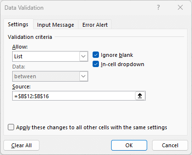
1. Data > Data Validation
2. Select Allow List
3. Select the range of of choices in the Source field

The resulting dialog should look a bit like this:

Hit OK, and now you have a drop-down in the cell:

With the Data Validation drop-down complete, we can move to the next exercise.

Bonus

If you don’t have a unique list of customers as shown above, you can have Excel create it for you based on transactions in the workbook.

One option, which would be good if the customer list is relatively static, is to copy/paste the customer name column from the data transactions into a single column and then use the Data > Remove Duplicates command to remove duplicates. You can also sort them by using Data > Sort.

Another option, which would be good if the transactions are stored in a Table and you want Excel to update the list each time the Table data changes, is to use the UNIQUE function on the Table’s Customer column, like this:

=UNIQUE(TableName[ColumnName])

To use these results in the drop-down, we use data validation to create a list with a source of =$A$1#. Note the spill operator # follows the absolute cell reference which points to the cell that contains the formula. You can also sort the list returned by the UNIQUE function by wrapping a SORT function around it, like SORT(UNIQUE()).

Note: the UNIQUE and SORT functions are not available in all Excel versions.

Exercise 2: Name the Selected Cell

To easily reference the customer selected, we’re going to assign a name to the cell that contains the drop-down. Here’s how:

1. Select the cell
2. Navigate to the Name Box (it is just to the left of the formula bar)
3. Type in the desired name, like Customer, and avoid spaces and funky characters
4. Hit Enter

Now that our cell is named Customer, we can refer to the cell via this name within our formulas.

With the drop-down created, and the cell named Customer, it is time to head to the next exercise.

Exercise 3: Apply Conditional Formatting

Now, moving on to the main step – setting up conditional formatting based on the selected customer.

Once a user selects a customer from the drop-down, we want transactions in another worksheet to be highlighted, like this:

To apply such conditional formatting to the data transactions:

1. Select the entire transactions range
2. Home > Conditional Formatting > New Rule
3. In the resulting dialog, select Use a formula to determine which cells to format
4. The formula will compare each row within the selected range to the customer selected in the drop-down. This will use a format like this: =$A1=Customer. Where $A1 is replaced with an absolute column that refers to the matching customer column, and a relative row reference that points to the row of the active cell. Customer is the defined name that points to the drop-down cell. Note that you create an absolute column reference to the customer column by preceding it with a dollar sign, like this: $A1.
5. Finally, set the formatting you want applied when the condition is met, and click OK.

The conditional formatting rule will look a bit like this:

Voila! We’ve linked our data validation with conditional formatting. By changing the customer selection in the drop-down list, Excel automatically highlights matching customers on the other sheet.

To summarize, Excel provides the convenience to combine conditional formatting and data validation, granting a visual way of tracking data across worksheets based on the selection made.

If you have any alternatives, enhancements, or questions, please post in the comment section below … thanks!

Sample file

Here’s a downloadable sample file that showcases this powerful technique:

Frequently Asked Questions

Q: Can I use conditional formatting with data validation in other scenarios?

Absolutely! While this post uses the customer scenario as an example, you can apply the same principles in myriad ways in Excel.

Q: Can I type my choices for Data Validation?

Indeed, in addition to pointing the choices to a worksheet range, you can also type a list of choices … just separate the choices with commas.

Q: Can I change the formatting later?

Surely! You can change the conditional formatting rule and related formatting by going to Home > Conditional Formatting > Manage Rules. Then you can Edit the rule as desired.

Q: Can I import and use this on Google Sheets?

While the steps may differ, Google Sheets also supports data validation, named ranges, and conditional formatting.