Battle of Heavyweights: Round 6

Welcome to Round 6! In this round, we’ll discover how both functions behave when we insert a new worksheet column. In other words, does inserting a new worksheet column break the formula? Or, will it keep working? Let’s find out … the round begins now.

Round 6

We would like to retrieve some information from a data table. So, we enter the Item IDs into a worksheet:

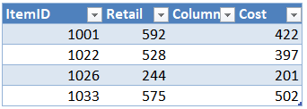
The data table (Table1) is here:

We’ll retrieve the Cost with both functions. Let’s start with VLOOKUP.

VLOOKUP

We write the following formula into C8:

=VLOOKUP(B8,Table1,3,FALSE)

We fill the formula down:

So far so good. But, what happens if we insert a new worksheet column between the lookup column (first column in the lookup range), and the return column (the column that has the value we are trying to return)? For example, let’s say we insert a new column into the data table to make room for a wholesale price:

Hmmm … our formula breaks:

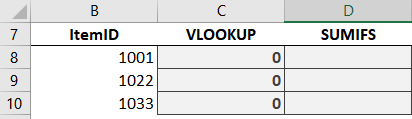
Now it returns 0 instead of the cost. Why? Because the 3rd argument is a whole number instead of a range reference. Let’s unpack this for a moment.

Normally, we can insert rows or columns as desired and formulas seem to just adapt. And Excel actually does an amazing job at this. I mean, just think about all of the references that have to be updated in various formulas when we insert a new row or column. And most of the time, nothing breaks. This is because most of time we use cell or range references such as C6 or A1:D10. But, let’s look at our formula for a moment:

=VLOOKUP(B8, Table1, 3, FALSE)

Here, we see that the 3rd argument is 3, which represents the column that contains the value we are trying to return. So, when we inserted a new worksheet column, Excel did not rewrite the argument value. Excel did not change the 3 to a 4. Which means it is now returning the new column (column 3) instead of the cost column (now column 4).

So, VLOOKUP, unlike most other functions, will not automatically adapt to a new column inserted between the first (lookup column) and return column within the range.

Now, let’s see about SUMIFS.

SUMIFS

We write the following formula in D8:

=SUMIFS(Table1[Cost],Table1[ItemID],B8)

We fill the formula down:

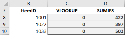
We can insert columns as desired, and nothing breaks. It still returns the cost. Why? Because we specifically identified the cost column Table1[Cost]. And, even if we had used ordinary range references like D6:D10 Excel would have updated it to E6:E10 when we inserted the column.

So, SUMIFS does not break when we insert a new worksheet column.

A note about XLOOKUP: The XLOOKUP function takes its cue from SUMIFS in this regard. That is, instead of using a col_index_num argument like VLOOKUP, XLOOKUP identifies the lookup and return columns independently like SUMIFS. This means that XLOOKUP won’t break when inserting new columns … yay!

Analysis

To recap our findings:

When we insert a new worksheet column between the lookup and return columns, VLOOKUP breaks whereas SUMIFS does not.

So, who won the round? Well, since this issue has broken many of my VLOOKUP functions over the years, I’d have to give the round to SUMIFS.

So, SUMIFS gets 10 points. And what about VLOOKUP? Can VLOOKUP accomplish this with a helper function? Depending on the structure of the workbook and labels, yes … this post shows how MATCH can help. So, VLOOKUP earns 9 points this round.

Scoreboard …

Updated stats …

See you in the next round!

Sample file: Round6.xlsx