Battle of Heavyweights: Round 3

Welcome to Round 3. In this round, we want to explore the idea of column order. That is, we want to find out if the order of the lookup table columns matter to these functions. Let’s find out! Round 3 … begins now!

Round 3

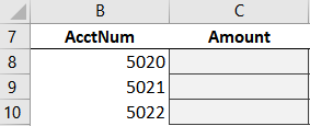
We are trying to build a little report, and we begin by entering a few account numbers into some cells:

Now, we’ll use a formula to retrieve the amounts from our data table (Table1), shown below:

Interesting … the first column is the Amount, not the AcctNum. Will this matter? Let’s start with VLOOKUP.

VLOOKUP

We write the following formula into C8:

=VLOOKUP(B8, Table1, 1, 0)

We fill the formula down, and hmmm:

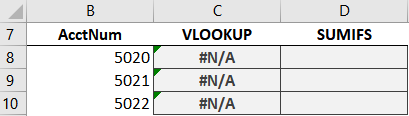
We get a bunch of errors. Why? After all, the second argument (Table1) defines the lookup table. And, the account number 5020 is in there!

Here’s the deal: when VLOOKUP is trying to find a matching value … it looks in the first column only. Once it finds a match, then it shoots to the right to retrieve the related value. But, while it is searching for the lookup value, it looks in the left-most column only (not the entire table).

So, column order does matter to VLOOKUP. What about SUMIFS? Let’s find out.

Note: column order doesn’t matter to XLOOKUP

SUMIFS

We write the following formula into D8:

=SUMIFS(Table1[Amount], Table1[AcctNum], B8)

We fill it down, and bam:

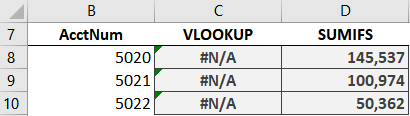
It works! Since we specify each column independently with SUMIFS, the column order does not matter.

Analysis

To recap what we’ve learned in this round:

Column order matters to VLOOKUP; not to SUMIFS

And, not only does the lookup column need to be the first column within the lookup range (table_array), the return column is expected to lie to the right of the lookup column. That is, VLOOKUP is designed to find a matching row and then shoot to the right to retrieve the related value.

So, if you encounter a similar workbook in practice, which function would you use? Me too … SUMIFS again!

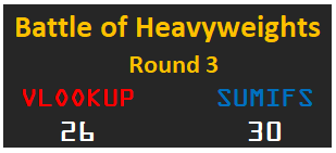
For points, SUMIFS gets 10. And, what about VLOOKUP. Can VLOOKUP accomplish this task with a helper function? Technically, yes. Here is a post that shows a clever way to use the CHOOSE function. So, we’ll give 9 points to VLOOKUP.

Updated scoreboard …

Updated stats …

I’ll see you in the next round!

Sample file: Round3.xlsx