Use Get & Transform to Reconcile Two Lists
In this post, we’ll use a Get & Transform query to help with our reconciliation. The idea for this post came from a question from Laura (thanks Laura!) The basic idea is that we have two worksheets. One contains the invoice totals and the other contains line item details, where there are many line items per invoice.
This is a basic reconciliation project, where we want to know if any invoices on the summary do not appear on the detail, and, if any invoice totals do not agree to the sum of the line items. Sound like a big, tedious project? Not with a Get & Transform query! Check it out.
Objective
Before we get to the mechanics, let’s just be sure we understand the details of our task.
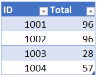
In one worksheet, we have a list of invoice totals. This invoice summary, stored in a table name SummaryTable, is shown below.
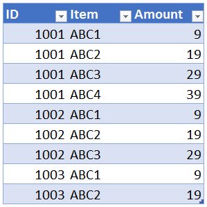
In another worksheet, we have stored the invoice line item details in a table named DetailTable, shown below.
We have a couple of goals with this reconciliation. First, we want to identify any invoices that appear on the summary but not on the detail. For example, invoice 1004 is on the summary but not the detail. Next, we want to compare the totals between both lists, and identify any invoices where the total on the summary does not tie to the sum of the line item details.
Since this is Excel, there are several approaches to accomplish this task. In this post, we’ll use a Get & Transform query to automate this reconciliation, not only for this month, but for all future months.
Details
The basic steps to prepare the reconciliation worksheet are:
- Create the summary query
- Create the detail query
- Create the reconciliation query
Let’s get to it.
Note: The steps below are presented with Excel for Windows 2016. If you are using a different version of Excel, please note that the features presented may not be available or you may need to download and install the Power Query Add-in.
Create the summary query
To create the summary query, click any data cell in the range, and click the Data > From Table ribbon icon. If the data is already stored in a table, as ours is, the Query Editor will open. If the data is in an ordinary range, then Excel will prompt you to create the table first.
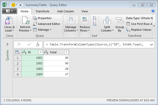
We confirm that the invoice summary data made it into the Query Editor, as shown below.
Since our data is ready to go, we don’t need to perform any transformations. If the data you are working with needs to be cleaned up, you can easily remove columns, add filters, or perform any additional transformations needed.
When the data is looking good, we use the Home > Close & Load DROP-DOWN (not the Close & Load button), and then select Close & Load To.

In the resulting Load To dialog, we select Only Create Connection and then click Load. We select this option because we don’t want the query results returned to cells in the workbook, but, we want to be able to access the results in another query (in our upcoming reconciliation query).
Create the detail query
Now, we need to create the detail query. To do this, we select any data cell in the range, and select Data > From Table.
The data flows into the Query Editor, as shown below.

Our data needs to be aggregated by ID. So, first, we’ll remove the Item column. To do this, we right-click the Item column header and select Remove.
Next, we need to create one row for each ID and compute the related sum. So, we right-click the ID column header and select Group By. Excel displays the Group By dialog, where we confirm that the Group by field is ID, and that we want to create a new column named Total that sums the Amount column, as shown below.

We click OK, and the updated results appear in the Query Editor, as shown below.

Our data is looking good, so we select Close & Load To, and once again select the Only Create Connection option in the Load To dialog.
At this point, our workbook contains a SummaryTable query and a DetailTable query as shown in the panel below.

The final step is to combine them and put the results into a new reconciliation worksheet.
Create the reconciliation query
To compare these queries, we select the Data > New Query > Combine Queries > Merge command.
In the resulting Merge dialog, we select SummaryTable from the first drop-down and DetailTable from the second drop-down. Then, we need to tell Excel which field is the common field between them. We do this by clicking the ID column from both preview windows. This is shown below.

We are just about done. The final decision is how Excel should join the two tables. We specify this with the Join Kind drop-down. In our reconciliation, we want our final reconciliation to include all invoices in the summary even if the invoice does not appear in the detail table. So, the default Left Outer join is perfect. There are many additional options that you can choose, for example, include all items in the detail even if they don’t appear on the summary (Right Outer), include all invoices from both lists (Full Outer), or only include invoices that appear on both lists (Inner). Once we pick the Join Kind, we click OK.
The Query Editor shows the results of the merge, as shown below.

Next, we need to tell Excel to display columns from the DetailTable, so, we click the icon in the NewColumn header and pick Expand (or alternatively, the Transform > Structured Column > Expand icon). We pick which columns to display, in our case, we’ll pick both the ID and Total columns and click OK.
The updated results are shown below.

So far, we can easily identify which invoices in the summary do not appear in the detail because of the null value. Now, we just need to make it easy to compare the two totals. We’ll do this by computing the difference between the two Total columns.
We create a new calculated column by clicking the Add Column > Custom Column icon. The Add Custom Column dialog is shown below.

Our new column name is Diff, and to create the formula we double-click the Total column in the Available Columns list, type a subtraction operator (-) and then double-click the NewColumn.Total column. We click OK, and the new column will be displayed in the Query Editor, as shown below.

Since we want to see the results of this query in Excel, we click the Close & Load command. The results appear in Excel as shown below.

At this point, the fun part of the reconciliation process is over. Now begins the not-so-fun part where we have to dig into the details and understand why certain invoices don’t appear on the detail sheet, like invoice 1004, and why some have a different amount (like invoice 1002).
Update Next Period
Now, this may feel like many steps to get our reconciliation generated. But, the benefit of investing the time is that the reconciliation will be generated in future periods very quickly by updating this workbook instead of creating a brand new reconciliation workbook. Simply paste the summary data into the existing SummaryTable, the detail data into the DetailTable, and then right-click and Refresh the green results table. Excel instantly generates an updated reconciliation table, without any need to open the Query Editor!
Note: If the structure of the data changes, or you want to update the Join Kind or transformations, you can open the Query Editor to update, but, when the basic structure is the same, you are good to go.
If you have any other fun approaches to reconciliations, or any other fun Get & Transform query tips, please share by posting a comment below…thanks!
Resources
- Download Excel file: ReconList.xlsx
Excel is not what it used to be.
You need the Excel Proficiency Roadmap now. Includes 6 steps for a successful journey, 3 things to avoid, and weekly Excel tips.
Want to learn Excel?
Our training programs start at $29 and will help you learn Excel quickly.
This is looking really good so far. I have used it with some small amounts of data that I had reconciled with another program. THANK YOU so much for going through this entire process. I really appreciate it.
Welcome and thanks again for the idea 🙂
I have also used it successfully with two lists that I set up as the detail query you mentioned above.
Beautiful 🙂
Thank you so much, I use Power Query for a lot of different functions, but usually to just combine data, but not to reconcile data. Look forward to when I have a project that I can use this on!
Thank you so much for these great tips!
Welcome…I absolutely LOVE this feature 🙂
Is this method better, faster, easier…than just using a sumif function on the totals sheet that references the detailed sheet and then subtracts the value shown on the total sheet. That way differences immediately pop out. Zero means it’s OK.
For a one-time project, a formula-based solution (such as with SUMIF or SUMIFS) is a nice alternative, assuming that all detailed transactions appear in the summary. The Get & Transform approach is fairly efficient for recurring-use workbooks because there are no helper columns to manage or update…it is just a right-click and Refresh. It is always fun to see that Excel offers multiple ways to accomplish any given task!
Thanks,
Jeff
Our payroll department has set up templates for 4 of their monthly reconciliations. I love being able to copy new data into the template, hit refresh and have a new reconciliation.
Totally awesome update, thanks!
Thanks Jeff, I always learn something new from you. Are you doing any California Education Foundation Classes on Power Query?
Sure am…it will be a new webinar this year. Look forward to “seeing” you there 🙂
I’m excited but when will it be, so I can mark my calendar now?
We are still working on the dates…thanks!
Power-full article.
Thank you so much, this is very helpful