Sum by Color
If you need to compute the total for certain cells based on their font or fill color, you may have noticed that Excel formulas operate on stored values, not displayed values. That means that functions such as SUM and SUMIFS operate on the underlying cell values and disregard cell formatting, such as font or fill color. This post provides three steps to workaround this issue and compute a total based on fill color.
Objective
Before we get too far, let’s have a look at what we are trying to accomplish.
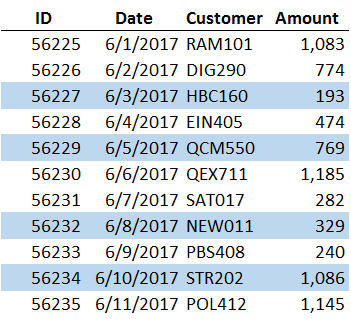
We have a range of data and selected transactions have been highlighted with a cell fill color, as shown below.
We’ll want to be able to highlight additional rows any time, and we don’t want to rewrite or update our formula when we do. That means our formula range needs to include the amount column and we are precluded from using a formula that picks and chooses each cell (like E10+E12+E15…).
When we try to write a formula that adds up the amount column but includes only the highlighted transactions, we get stuck. Regardless of which summing function we use, we can’t seem to tell Excel to include only the highlighted cells. This is because formulas operate on the underlying stored values and disregard the cell formatting.
So, can we do this? Yes, we can, no worries.
How To
We can accomplish our objective with the help of two Excel items, namely, a filter and a SUBTOTAL function.
Step 1: The filter. We can filter by font or fill color using the built-in filter feature of Excel. To turn on filters, simply select any cell within the data range and then the following Ribbon icon:
- Data > Filter
This will turn on little filter controls, or drop-downs, in the header row. These are shown below.
![]()
With them, we can filter by fill color. Simply pull one down, and then select Filter by Color. A slide-out menu will appear showing the colors used within the data region. When you pick a color, Excel will show those rows and hide the others, as demonstrated below.
Once we have the filter working, we are just about done. All we need to do is write a formula that includes only the visible rows.
Step 2: The blank row. Since we always want our total row to be visible, we don’t want it included within the filter range. To prevent Excel from hiding the total row when applying a filter, we want to skip a row before writing the formula. So, we won’t write our formula in the row immediately under the data range, we’ll leave a blank row in between the last data row and the formula row.
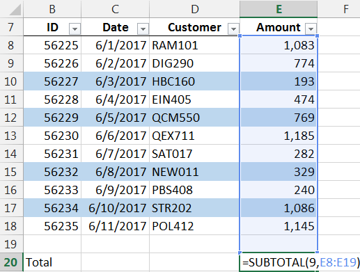
Step 3: SUBTOTAL. Excel has several functions that can add stuff up. To accomplish our objective, we can’t use a standard SUM function because it includes both visible and hidden rows. The SUBTOTAL function on the other hand, includes only visible rows within a filtered region. The trick to using the SUBTOTAL function is to set the first argument to either 9 or 109. Either would work in this case because we want to sum the results and we are using a filter to hide the rows. If our amount column was stored in the range E8:E19, then we would use the following formula in our total row:
=SUBTOTAL(9, E8:E19)
This is pictured below.
Connecting the dots then…we know we can use the filter to show only the highlighted transactions, we know the blank row between the last data row and the formula will help ensure that our total row is excluded from the filter, and we know the SUBTOTAL function will include only the visible rows within the filtered region. So, will this work? Let’s find out…
Yes, it worked! The total updates from 7,560 (all rows) to 2,377 (highlighted rows)…we have computed a total based on fill color just like we wanted!
If you have any other fun techniques for summing by color, or other suggested uses for filters, please share by posting a comment below…thanks!
Notes
- Download the Excel file: SumByColor
- This technique works if the data is stored in a table as well. Instead of writing the SUBTOTAL formula manually, Excel will add it automatically when we check the Total Row checkbox on the TableTools ribbon tab. Plus, the filter controls will automatically be included in the table’s header row.
- If your total row is being included the the filter (and thus hidden) be sure you have a blank row between the last data row and the formula row and then turn off filters (Data > Filter) and then back on again (Data > Filter).
Excel is not what it used to be.
You need the Excel Proficiency Roadmap now. Includes 6 steps for a successful journey, 3 things to avoid, and weekly Excel tips.
Want to learn Excel?
Our training programs start at $29 and will help you learn Excel quickly.
Clever 🙂 Thanks for this one. It was fun reading your post.
Love it!
This is great! I use color all the time and, before this trick, laboriously selected the cells to sum. Great time saver.
Glad this will help save some time 🙂
This image depicts that here we don’t need the total sum of all the elements but instead we want the sum of elements that have the same background color.
My only thing…i have 4000 rows that have to be displayed but only want to total the highlighted cells. Not have the total to change to accept all cells as demonstrated above.
Pamela
If all 4000 rows need to be displayed, and you want the total of a subset (the highlighted rows) then one option is to use a helper column with SUMIFS. For example, apply a temporary filter to display the highlighted rows. Then enter a stored value such as TRUE or Yes in the helper column for all visible (highlighted) rows. Then you can remove the filter to display all rows. At this point, you can use SUMIFS (or a PivotTable) to compute the sum based on the stored values in the helper column. I have a blog post that demonstrates the SUMIFS function in case it would help. https://www.excel-university.com/multiple-condition-summing-in-excel-with-sumifs/
Thanks
Jeff
Very helpful, I’m looking to do this with SUMPRODUCT, thus a very similar problem but with fixed values being multiplied by by a quantity in an adjacent column, Ideally using a macro.
I have a spreadsheet that contains paid and accrued totals in same column, as shown below. The accrued amounts are in red (representing negative $$) and the paid $$ are regular print (black). I want to write a formula that will automatically adjust the bottom line total if additional $$ (red or black) are added to a column. In other words, I want the formula to automatically adjust by color.
AMRI-07 October $1,640.94
AMRI-08 November $1,236.57
AMRI-09 December $1,131.30
AMRI-10 January $1,486.40
AMRI-12 March $2,626.23
AMRI-13 Apri $1,304.03
Accrual May -2,922.39 (color red)
Accrual June -12,774.67 (color red)
Accrual July-Sept -19,000.00 (color red)
In other words, if I add negative $$, the figure will automatically appear in red.
Hey Alice!
First, you would ideally have the numbers in an Excel Table, so that the formatting will apply to any additional rows in that column. Then you just need to adjust the number format to whatever you want. Highlight the column then click the format dialog box. (I prefer the keyboard shortcut Ctrl+1!) On the number tab, you’ll see numerous options, including even a custom format! You probably only need the currency or accounting option, and choose the black with the red negative number.
Hope that helps:)
Kurt LeBlanc
Is there a way to sum conditional formatted cells that have color? I have a spreadsheet that across the column headers are weekly dates, and then below that, sales data. When a product is on sale, it is highlighted in yellow, using conditional formatting.
I would like to just add up the yellow cells. This will encompass 52 columns by years end.
Thanks
Tim
I have come accross a way but requires some vbcode to identify cell colour to do it, alternative you can use one of the cell() formulas to pick the colour attribute and then use sumif or sumproduct.